
Contour plot of gradient of squared electric field strength, ∇E 2 rms
The electric field is said to be the gradient (as in grade or slope) of the electric potential. For continually changing potentials, Δ V Δ V and Δ s Δ s become infinitesimals and differential calculus must be employed to determine the electric field.
Electric Potential Electric Field as Potential Gradient
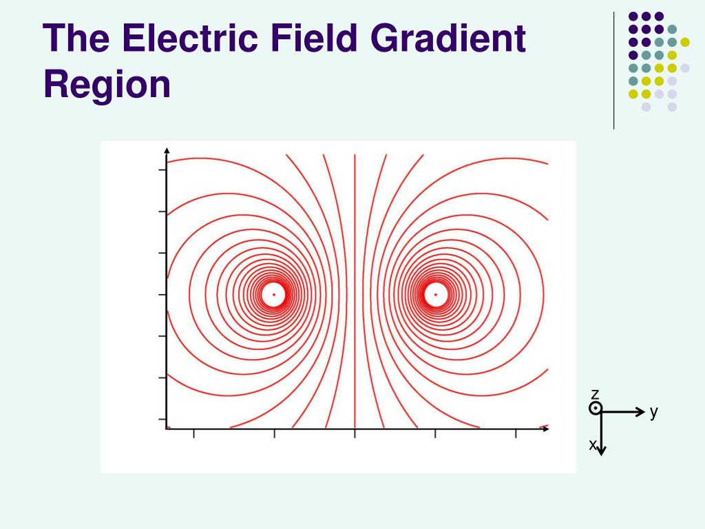
The electric field is the gradient of the potential. The gradient is in the direction of the most rapid change of the potential, and is therefore perpendicular to an equipotential surface. If $\FLPE$ were not perpendicular to the surface, it would have a component in the surface. The potential would be changing in the surface, but then it.
The gradient of electric field squared across the DEPwell C0 and the
Electric fields are caused by electric charges, described by Gauss's law, and time varying magnetic fields, described by Faraday's law of induction. Together, these laws are enough to define the behavior of the electric field. However. is the gradient of the electric potential and.

Electric Field as Potential Gradient FSc Class 12 PHYSICS Chapter
The gradient of a scalar field is a vector that points in the direction in which the field is most rapidly increasing, with the scalar part equal to the rate of change. A particularly important application of the gradient is that it relates the electric field intensity \({\bf E}({\bf r})\) to the electric potential field \(V({\bf r})\).
Calculating E from V(x,y,z) E = potential gradient Electrostatic
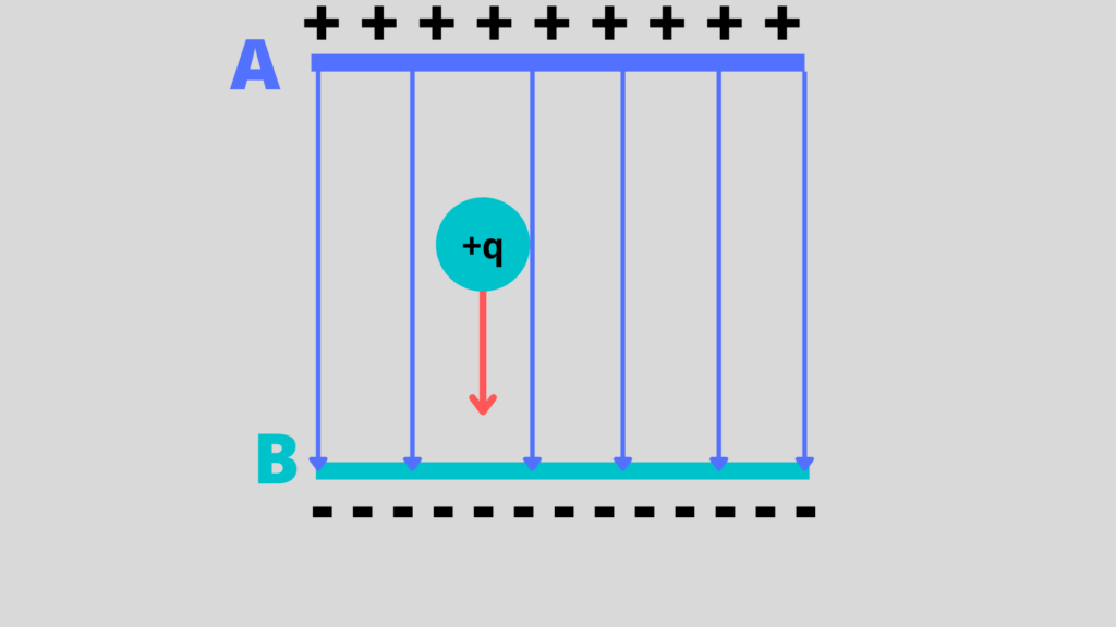
See the text for details.) The work done by the electric field in Figure 19.2.1 19.2. 1 to move a positive charge q q from A, the positive plate, higher potential, to B, the negative plate, lower potential, is. W = −ΔPE = −qΔV (19.2.1) (19.2.1) W = − Δ P E = − q Δ V. The potential difference between points A and B is.

Electric Field as potential gradient Class 12 ElectrostaticsNCERT
In vector calculus notation, the electric field is given by the negative of the gradient of the electric potential, E = − grad V. This expression specifies how the electric field is calculated at a given point. Since the field is a vector, it has both a direction and magnitude.
The simulation result of the electrical field and potential
Measurement(s) electric field gradient Technology Type(s) computational modeling technique Factor Type(s) material studied Machine-accessible metadata file describing the reported data: https.

Are All Electric Field The Gradient Of A Potential Dr Bakst
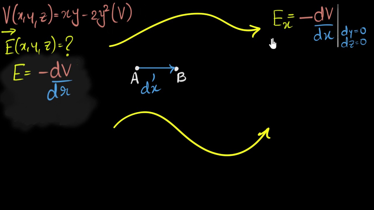
Relation between field & potential Calculating E from V (x,y,z): E = - potential gradient Google Classroom About Transcript Let's calculate the electric field vector by calculating the negative potential gradient. We first calculate individually calculate the x,y,z component of the field by partially differentiating the potential function.
a) Electric field gradient distribution at the tip region under DC bias
5.14: Electric Field as the Gradient of Potential. where E(r) E ( r) is the electric field intensity at each point r r along C C. In Section 5.12, we defined the scalar electric potential field V(r) V ( r) as the electric potential difference at r r relative to a datum at infinity. In this section, we address the "inverse problem.

Electric field gradient squared distribution on the surfaces of both
7.14. With this notation, we can calculate the electric field from the potential with. E→ = −∇ V, E → = − ∇ → V, 7.15. a process we call calculating the gradient of the potential. If we have a system with either cylindrical or spherical symmetry, we only need to use the del operator in the appropriate coordinates: Cylindrical:∇.

Relation Between Potential Gradient And Electric Field YouTube
The gradient of the electric field is the second derivative of the electrostatic potential, and as such, it obeys certain symmetries; The EFG is a symmetric tensor with zero trace.

Electric field as potential gradient 12th physics SWAJ Foundation
As shown in Figure 7.5.1, if we treat the distance Δs as very small so that the electric field is essentially constant over it, we find that. Es = − dV ds. Therefore, the electric field components in the Cartesian directions are given by. Ex = − ∂V ∂x, Ey = − ∂V ∂y, Ez = − ∂V ∂z. This allows us to define the "grad" or.

(a) Electric field gradient distribution (V/m), (b) 3D top view of the
A numerical model of oil-solid multi-gradient filtration with electric field enhancement was developed by coupling the electric field governing equation, flow field governing equations, discrete phase tracking equation, and particle-wall collision model equation.. When the electric field strength is 2 kV/mm, the inlet flow rate is 0.3 m.
a) 2D plot of norm of electric field gradient b) Norm of electric field
Droplet directional transport is one of the central topics in microfluidics and lab-on-a-chip applications. Selective transport of diverse droplets, particularly in another liquid phase environment with controlled directions, is still challenging. In this work, we propose an electric-field gradient-driven droplet directional transport platform facilitated by a robust lubricant surface. On the.

Finite element simulation with COMSOL; areas with different color
An electric field gradient is a measure of how the electric field changes with respect to position within a region of space. It is a vector quantity that describes the rate of change of the electric field in each direction.
PPT Measuring Polarizability with an Atom Interferometer PowerPoint
In atomic, molecular, and solid-state physics, the electric field gradient ( EFG) measures the rate of change of the electric field at an atomic nucleus generated by the electronic charge distribution and the other nuclei.
